User’s Guide#
The ccf_streamlines Python package presents an interface to use the isocortical
streamlines of the Allen Mouse Common Coordinate Framework (CCF). These
streamlines can be used to visualize three-dimensional CCF-aligned data from the mouse
isocortex in flattened or two-dimensional representations, as well as to align
data in a consistent pia/white matter orientation.
The CCF is a high resolution, three-dimensional reference atlas for the mouse brain. For more information about the CCF, please refer to its technical white paper reference and the publication by Wang et al. (2020). You can access the Allen CCF at atlas.brain-map.org.
One note of caution - the 3D data files and streamline reference files are fairly large, given the high resolution and size of the Allen CCF. The package has been written to attempt to minimize its memory footprint, but you still may encounter memory issues depending on the capabilities of your machine, how many data sets or projections you try to use at once, etc.
What are streamlines?#
Streamlines are the paths that most directly connect the pia of the isocortex to the white matter while following the curvature of those surfaces. As the CCF white paper states:
After the borders of isocortex were defined, Laplace’s equation was solved between pia and white matter surfaces resulting in intermediate equi-potential surfaces (Figure 4A). Streamlines were computed by finding orthogonal (steepest descent) path through the equi-potential field (Figure 4B). Information at different cortical depths can then be projected along the streamlines to allow integration or comparison.
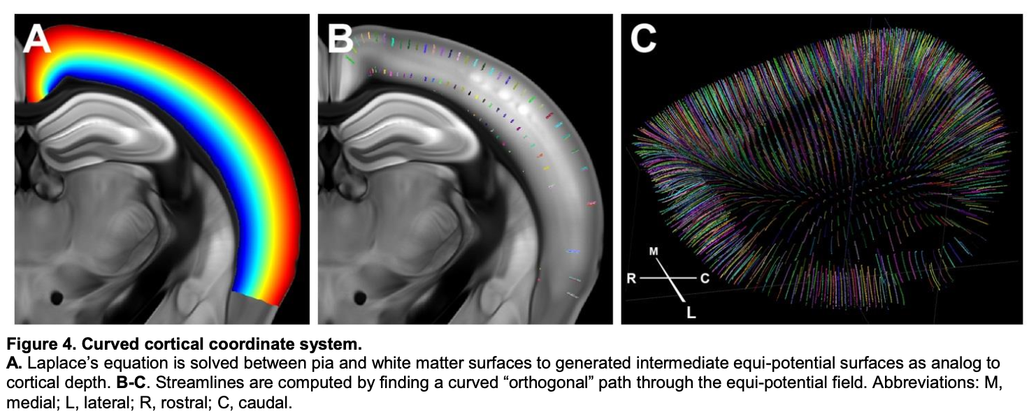
In practice, these streamlines are connected sets of voxels in the 3D CCF space. By their nature, streamlines link voxels within the isocortex to voxels at the pial surface. These surface voxels can be visualized in two-dimensions, either by recreating views of the curved surface from various perspectives (e.g., from looking down on top, or by looking from the side) or by flattening the isocortex so that the entire surface can be visualized as one sheet. Accordingly, you can use the streamlines to determine which voxels in the 3D space should contribute each location in the 2D projections.
Projecting a volume to 2D#
This section will present how to use the ccf_streamlines package to project
3D CCF-aligned data to two-dimensional views. As an example, we will use the
10-micron resolution average template data for the CCF.
(note: this file is ~300 MB). The file is in the NRRD format.
After downloading the file to the director we’re working in, we can load it into a 3D NumPy array.
import nrrd
import numpy as np
import matplotlib.pyplot as plt

template, _ = nrrd.read("average_template_10.nrrd")
Now, we can set up our projector object to perform operations on this 3D data.
We’ll first need a few other files, which you can find listed in Data Files.
For this example, we’ll be using the top.h5 view lookup file and the
surface_paths_10_v3.h5 streamlines file. These will be given to a
Isocortex2dProjector object that will
process the 3D data.
import ccf_streamlines.projection as ccfproj

proj_top = ccfproj.Isocortex2dProjector(
    # Specify our view lookup file
    "top.h5",

    # Specify our streamline file
    "surface_paths_10_v3.h5",

    # Specify that we want to project both hemispheres
    hemisphere="both"

    # The top view contains space for the right hemisphere, but is empty.
    # Therefore, we tell the projector to put both hemispheres side-by-side
    view_space_for_other_hemisphere=True,
)
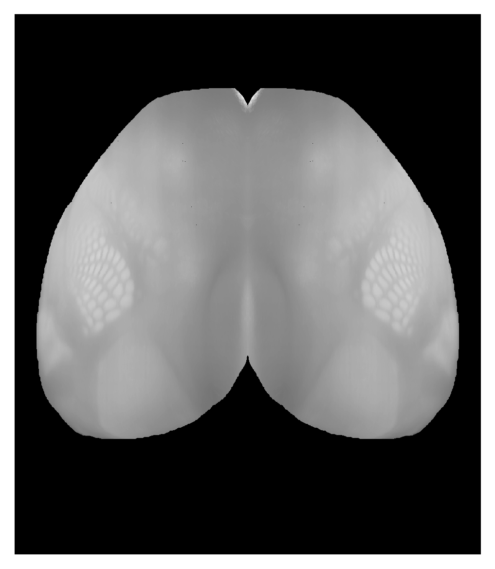
We can now project the volume to a 2D top view. The default way of consolidating the information along the streamline is to use a maximum intensity projection (so the highest value along the streamline is used in the 2D image).
top_projection_max = proj_top.project_volume(template)

plt.imshow(
    top_projection_max.T, # transpose so that the rostral/caudal direction is up/down
    interpolation='none',
    cmap='Greys_r',
)
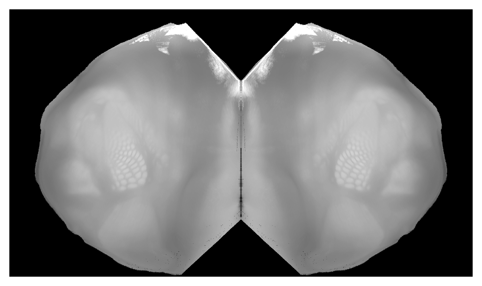
If we wanted to use a different view file (such as the “butterfly” flat map), we would just pass that as a different configuration option.
proj_bf = ccfproj.Isocortex2dProjector(
    # Specify our view lookup file
    "flatmap_butterfly.h5",

    # Specify our streamline file
    "surface_paths_10_v3.h5",

    # Specify that we want to project both hemispheres
    hemisphere="both",

    # The butterfly view doesn't contain space for the right hemisphere,
    # but the projector knows where to put the right hemisphere data so
    # the two hemispheres are adjacent if we specify that we're using the
    # butterfly flatmap
    view_space_for_other_hemisphere='flatmap_butterfly',
)

bf_projection_max = proj_bf.project_volume(template)

plt.imshow(
    bf_projection_max.T, # transpose so that the rostral/caudal direction is up/down
    interpolation='none',
    cmap='Greys_r',
)
Since the CCF is an annotated reference atlas, we also know which isocortical
region each surface voxel belongs to. It is often useful to draw the region
boundaries on top of the projected images, and we can use the BoundaryFinder
object to do so. (We’ll need the appropriate atlas files from Data Files
to do this, too.)
bf_boundary_finder = ccfproj.BoundaryFinder(
    projected_atlas_file="flatmap_butterfly.nrrd",
    labels_file="labelDescription_ITKSNAPColor.txt",
)

# We get the left hemisphere region boundaries with the default arguments
bf_left_boundaries = bf_boundary_finder.region_boundaries()

# And we can get the right hemisphere boundaries that match up with
# our projection if we specify the same configuration
bf_right_boundaries = bf_boundary_finder.region_boundaries(
    # we want the right hemisphere boundaries, but located in the right place
    # to plot both hemispheres at the same time
    hemisphere='right_for_both',

    # we also want the hemispheres to be adjacent
    view_space_for_other_hemisphere='flatmap_butterfly',
)
These boundaries are returned as dictionaries with the region acronyms as the keys and the values as 2D arrays of the boundary coordinates (in the space of the projection).
bf_left_boundaries
{'ACAd': array([[1100.5,  592. ],
        [1100. ,  591.5],
        [1099.5,  591. ],
        ...,
        [1099.5,  593. ],
        [1100. ,  592.5],
        [1100.5,  592. ]]),
 'ACAv': array([[1176.5,  704. ],
        [1176. ,  703.5],
        [1175.5,  703. ],
        ...,
...
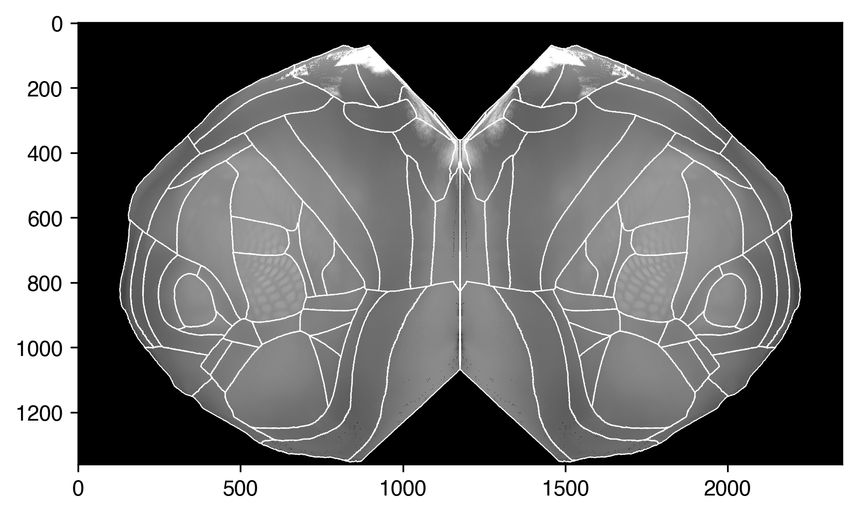
Now we can plot them on top of the average template projection.
plt.imshow(
    bf_projection_max.T,
    interpolation='none',
    cmap='Greys_r',
)

for k, boundary_coords in bf_left_boundaries.items():
    plt.plot(*boundary_coords.T, c="white", lw=0.5)
for k, boundary_coords in bf_right_boundaries.items():
    plt.plot(*boundary_coords.T, c="white", lw=0.5)
Projecting a volume to 3D “slab”#
For the “flatmap” projection types, we could imagine them as taking the isocortical surface and pressing it flat (rather than simply viewing the cortex from different angles, as with the other view types). In this case, we may be interested not only in viewing our data across the cortical surface, but also throughout the (flattened) cortical depth.
We’ll use an Allen Mouse Brain Connectivity Atlas as an example, since we’ll be able to see processes that travel perpendicular to the cortical surface (e.g., apical dendrites of labeled neurons).
We’ll look at this experiment in which cells labeled by the Tlx-Cre driver (primarily excitatory neurons in layer 5a of cortex) in the visual area VISal are fluorescent. You can download the projection data with this link:
http://api.brain-map.org/grid_data/download_file/297231636??image=projection_density&resolution=10
Once that is downloaded, we will load it as we did the average template.
tlx_data, _ = nrrd.read("11_wks_coronal_297231636_10um_projection_density.nrrd")
Since we want to preserve the depth information, we’ll use a Isocortex3dProjector
object. We also are going to normalize the thickness of each layer to a precalculated
set of thicknesses, so we’ll need a few additional files from Data Files
to set up our projector.
We’ll load that depth information from a JSON file first.
import json

# Note - the layer depths in this file was calculated from a set of visual cortex slices,
# so you may wish to use another set of layer depths depending on your purposes

with open("avg_layer_depths.json", "r") as f:
    layer_tops = json.load(f)

layer_thicknesses = {
        'Isocortex layer 1': layer_tops['2/3'],
        'Isocortex layer 2/3': layer_tops['4'] - layer_tops['2/3'],
        'Isocortex layer 4': layer_tops['5'] - layer_tops['4'],
        'Isocortex layer 5': layer_tops['6a'] - layer_tops['5'],
        'Isocortex layer 6a': layer_tops['6b'] - layer_tops['6a'],
        'Isocortex layer 6b': layer_tops['wm'] - layer_tops['6b'],
}
And then configure our projector. Because they require more data and calculation, both setting up and using the projector are more time and resource intensive in 3D.
proj_butterfly_slab = ccfproj.Isocortex3dProjector(
    # Similar inputs as the 2d version...
    "flatmap_butterfly.h5",
    "surface_paths_10_v3.h5",

    hemisphere="both",
    view_space_for_other_hemisphere='flatmap_butterfly',

    # Additional information for thickness calculations
    thickness_type="normalized_layers", # each layer will have the same thickness everwhere
    layer_thicknesses=layer_thicknesses,
    streamline_layer_thickness_file="cortical_layers_10_v2.h5",
)
Once we have it set up, we can project the data in the same was as in 2D.
tlx_normalized_layers = proj_butterfly_slab.project_volume(tlx_data)
We can plot max intensity projections of the view from the top, as we did before. But we can also look at our “slab” from the side.
# Calculate our maximum intensity projections of the slab
# and keep track of their shapes (to set up the plots to be right size

main_max = tlx_normalized_layers.max(axis=2).T
top_max = tlx_normalized_layers.max(axis=1).T
left_max = tlx_normalized_layers.max(axis=0)

main_shape = main_max.shape
top_shape = top_max.shape
left_shape = left_max.shape


# Set up a figure to plot them together
fig, axes = plt.subplots(2, 2,
                         gridspec_kw=dict(
                             width_ratios=(left_shape[1], main_shape[1]),
                             height_ratios=(top_shape[0], main_shape[0]),
                             hspace=0.01,
                             wspace=0.01),
                         figsize=(19.4, 12))

# Plot the surface view
axes[1, 1].imshow(main_max, vmin=0, vmax=1, cmap="magma", interpolation=None)

# plot our region boundaries
for k, boundary_coords in bf_left_boundaries.items():
    axes[1, 1].plot(*boundary_coords.T, c="white", lw=0.5)
for k, boundary_coords in bf_right_boundaries.items():
    axes[1, 1].plot(*boundary_coords.T, c="white", lw=0.5)

axes[1, 1].set(xticks=[], yticks=[], anchor="NW")

# Plot the top view
axes[0, 1].imshow(top_max, vmin=0, vmax=1, cmap="magma", interpolation=None)
axes[0, 1].set(xticks=[], yticks=[], anchor="SW")

# Plot the side view
axes[1, 0].imshow(left_max, vmin=0, vmax=1, cmap="magma", interpolation=None)
axes[1, 0].set(xticks=[], yticks=[], anchor="NE")

# Remove axes from unused plot area
axes[0, 0].set(xticks=[], yticks=[])
sns.despine(ax=axes[0, 0], left=True, bottom=True)
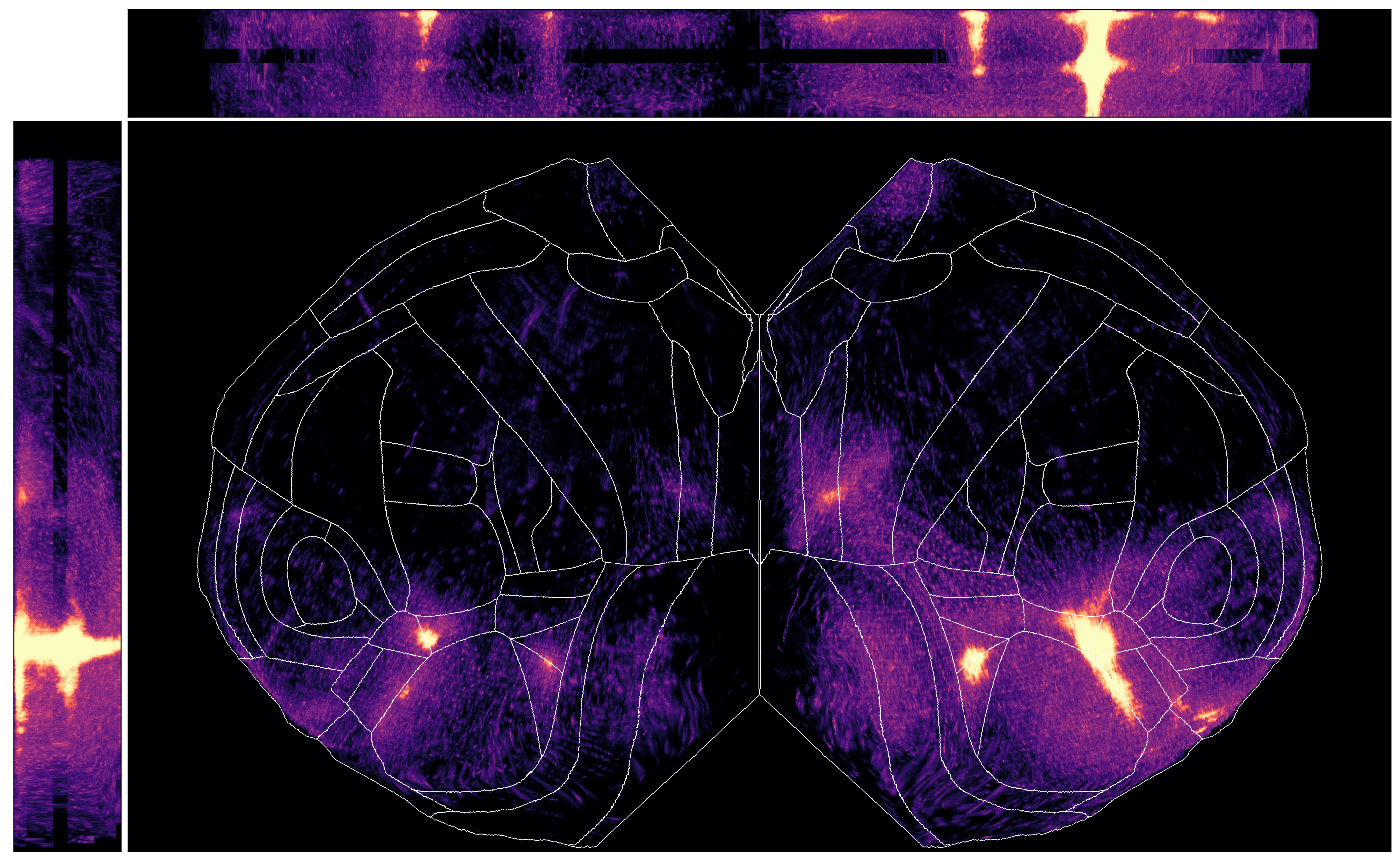
You may notice certain “gaps” in the data - this is because we have normalized
to a consistent layer thickness, but layer 4 is not present in all areas in the
CCF. In those areas, those parts of the slab are left empty, so the data will
look like they “skip” across. This only occurs with the normalized_layers option
to the thickness_type parameter.
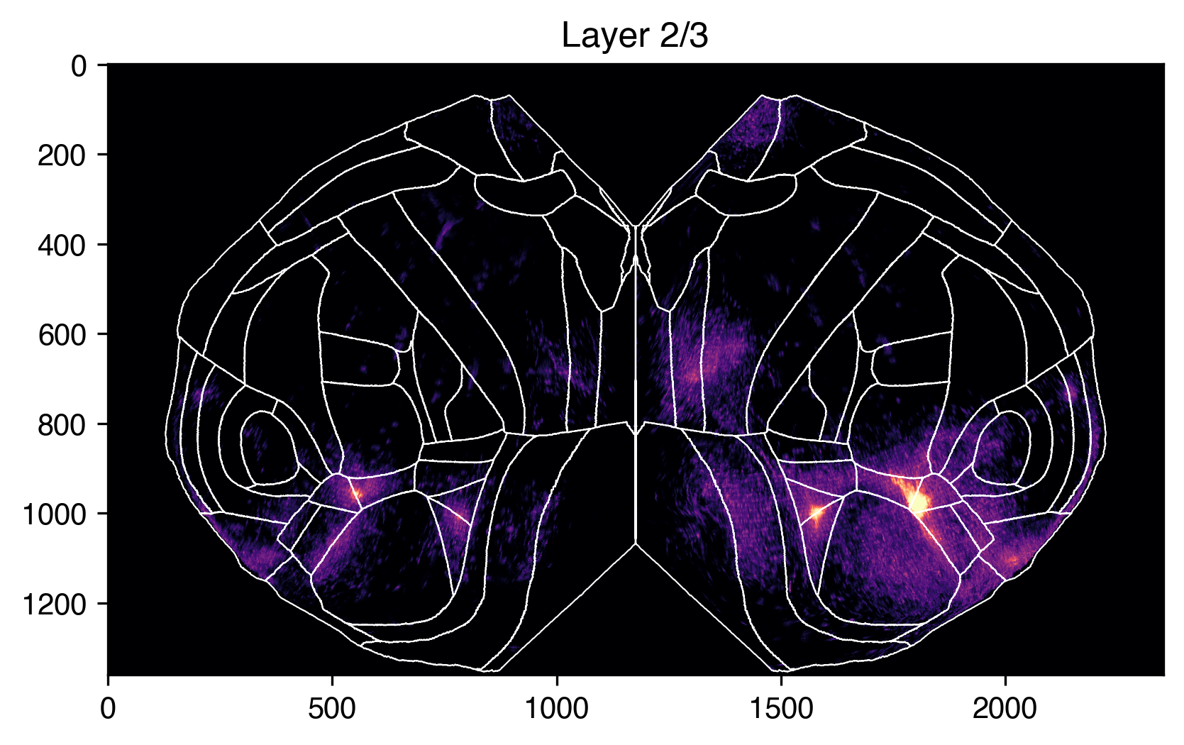
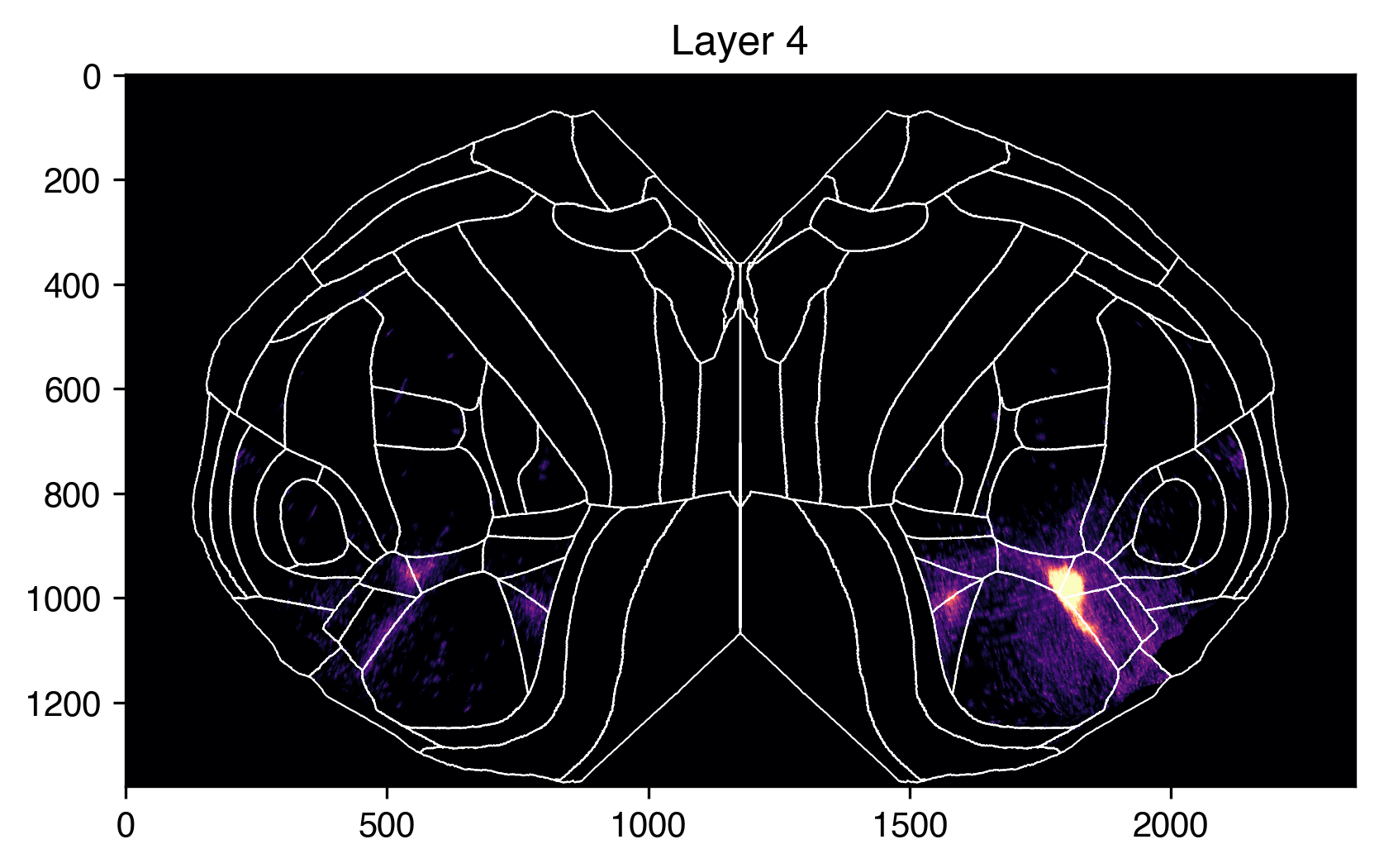
Because our slab is 3D, we can also look at sections of it at different depths. For example, we can compare L2/3 to L4 like so.
# find the max projection of just layer 2/3
plt.figure()
plt.imshow(
    tlx_normalized_layers[:, :, top_l23:top_l4].max(axis=2).T,
    vmin=0, vmax=1,
    cmap="magma",
    interpolation=None
)

# plot region boundaries
for k, boundary_coords in bf_left_boundaries.items():
    plt.plot(*boundary_coords.T, c="white", lw=0.5)
for k, boundary_coords in bf_right_boundaries.items():
    plt.plot(*boundary_coords.T, c="white", lw=0.5)

plt.title("Layer 2/3")


# find the max projection of just layer 4
plt.figure()
plt.imshow(
    tlx_normalized_layers[:, :, top_l4:top_l5].max(axis=2).T,
    vmin=0, vmax=1,
    cmap="magma",
    interpolation=None
)

# plot region boundaries
for k, boundary_coords in bf_left_boundaries.items():
    plt.plot(*boundary_coords.T, c="white", lw=0.5)
for k, boundary_coords in bf_right_boundaries.items():
    plt.plot(*boundary_coords.T, c="white", lw=0.5)

plt.title("Layer 4")
Projecting a volume using all the streamlines#
The 2D projection files arrange the data from streamlines in a spatially organized way, as if by either viewing the cortex from a particular direction or by flattening it to see as much of the cortex from a single perspective. However, this means that any given view (even the flattened views) does not include every streamline of the isocortex.
Instead, we can use the
IsocortexEntireProjector to perform summary
operations on every streamline for a given input volume. This returns a linear
array of summarized values, and the class can also return a list of 3D coordinates
from the top of each streamline in the same order, so that every value can be
linked to a location on the cortical surface.
# We only need to provide the streamline file since we are not using
# any 2D view lookup
proj_entire = ccfproj.IsocortexEntireProjector("surface_paths_10_v3.h5")

# Sum all the values for every streamline
sum_vals = proj_entire.project_volume(tlx_data, kind='sum')

# Get the coordinates for the top of every streamline (in the same
# order as sum_vals)
streamline_coords = proj_entire.top_of_streamline_coords()
We can visualize the result as a 3D scatter plot:
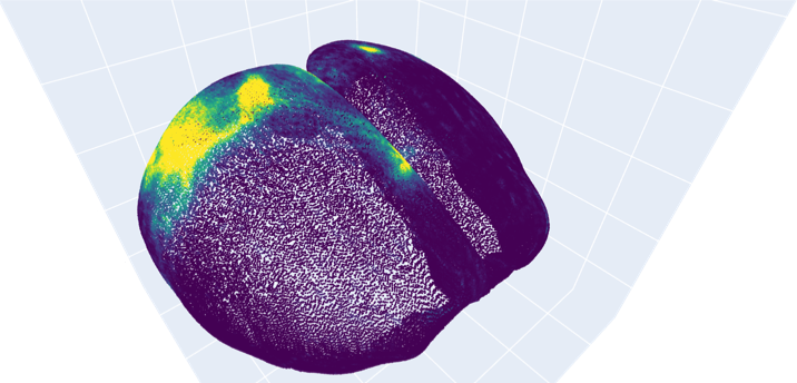
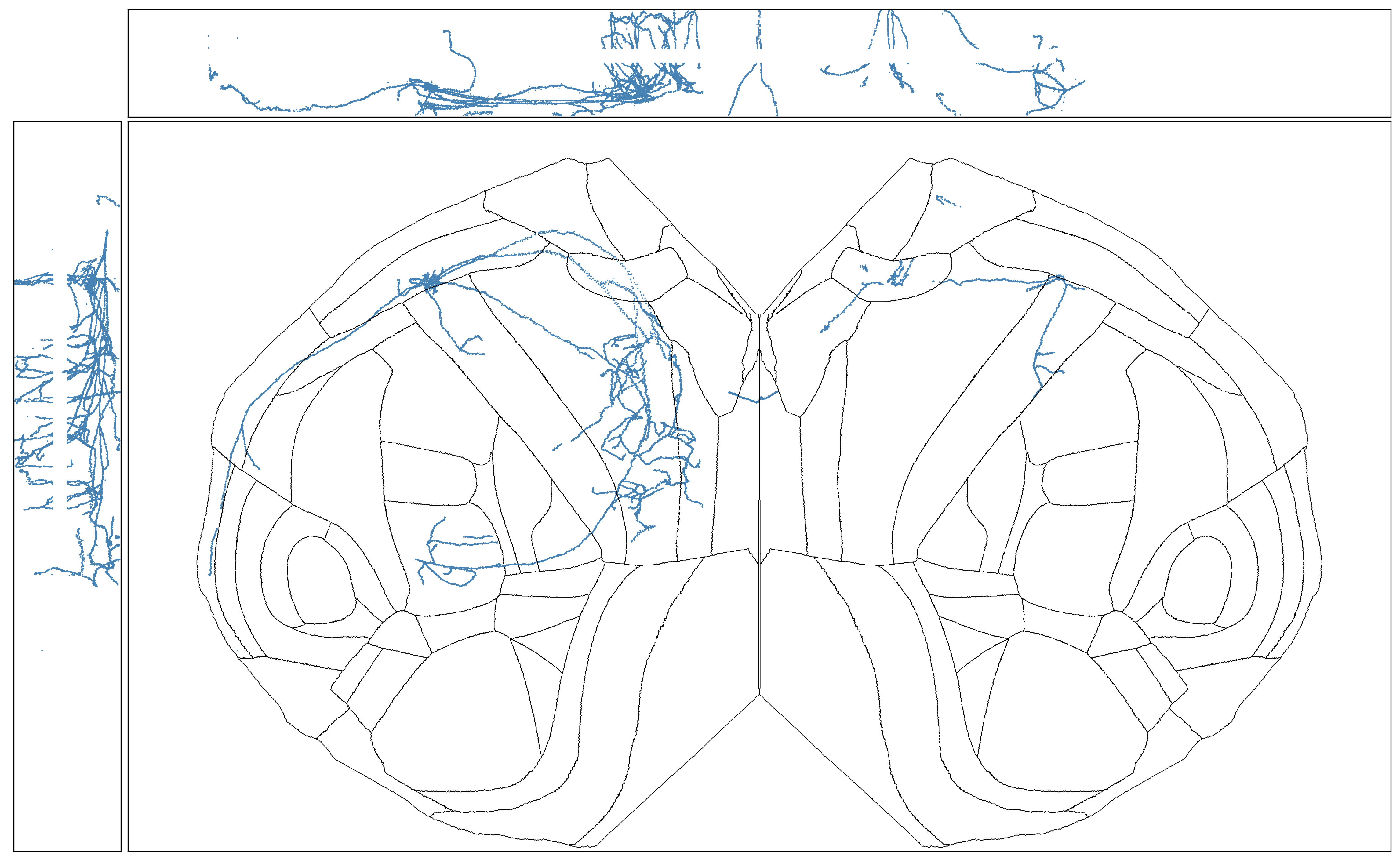
Projecting a morphology to 3D “slab”#
We can also use ccf_streamlines to look at CCF registered single neuron
morphologies in flattened representations. We can download an example morphology
from the study Peng et al. (2021),
from which the data can be downloaded here
We’ll use the neuron 17782_3284_X11909_Y16428 as an example, which can
be downloaded at this address:
We can use the morphological data in two ways. First, we’ll convert it into a
3D volume of the same kind we’ve been using so far. Then, we can use the same
tools to produced the flattened representations. To do this, we’ll use the function
transform_swc_to_volume().
import ccf_streamlines.morphology as ccfmorph

swc_file = "1119749935_17782_3284-X11909-Y16428_reg.swc"
morph_vol = ccfmorph.transform_swc_to_volume(swc_file)
Now we can pass this to our projector objects as before.
morph_normalized_layers = proj_butterfly_slab.project_volume(morph_vol)
# Calculate our maximum intensity projections of the slab
# and keep track of their shapes (to set up the plots to be right size

main_max = morph_normalized_layers.max(axis=2).T
top_max = morph_normalized_layers.max(axis=1).T
left_max = morph_normalized_layers.max(axis=0)


# Same plotting code as before...
main_shape = main_max.shape
top_shape = top_max.shape
left_shape = left_max.shape

# Set up a figure to plot them together
fig, axes = plt.subplots(2, 2,
                         gridspec_kw=dict(
                             width_ratios=(left_shape[1], main_shape[1]),
                             height_ratios=(top_shape[0], main_shape[0]),
                             hspace=0.01,
                             wspace=0.01),
                         figsize=(19.4, 12))

# Plot the surface view
axes[1, 1].imshow(main_max, vmin=0, vmax=1, cmap="Blues", interpolation=None)

# plot our region boundaries
for k, boundary_coords in bf_left_boundaries.items():
    axes[1, 1].plot(*boundary_coords.T, c="black", lw=0.5)
for k, boundary_coords in bf_right_boundaries.items():
    axes[1, 1].plot(*boundary_coords.T, c="black", lw=0.5)

axes[1, 1].set(xticks=[], yticks=[], anchor="NW")

# Plot the top view
axes[0, 1].imshow(top_max, vmin=0, vmax=1, cmap="Blues", interpolation=None)
axes[0, 1].set(xticks=[], yticks=[], anchor="SW")

# Plot the side view
axes[1, 0].imshow(left_max, vmin=0, vmax=1, cmap="Blues", interpolation=None)
axes[1, 0].set(xticks=[], yticks=[], anchor="NE")

# Remove axes from unused plot area
axes[0, 0].set(xticks=[], yticks=[])
sns.despine(ax=axes[0, 0], left=True, bottom=True)
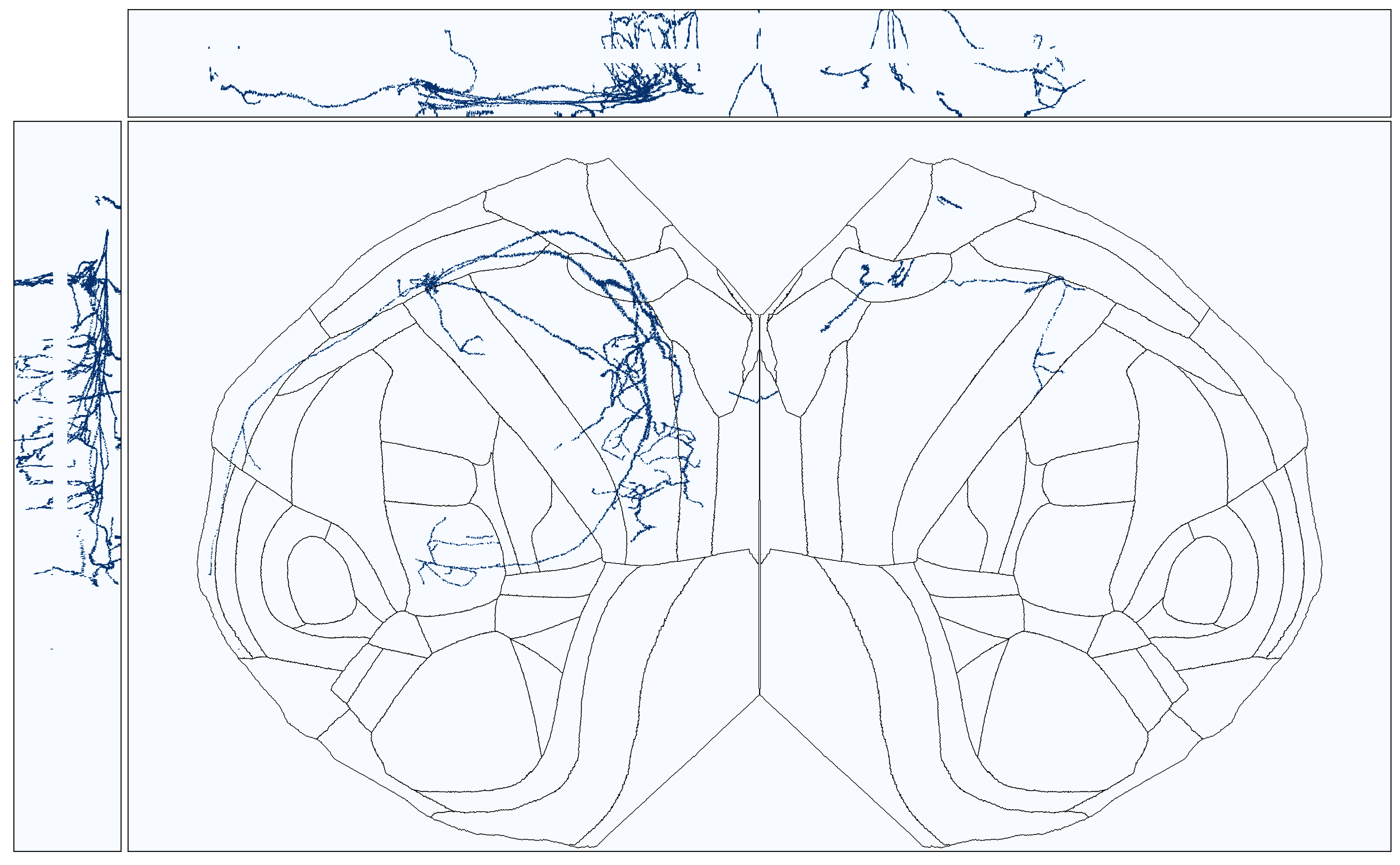
We could also transform each coordinate of the reconstructed morphology to our
flattened space instead of converting the morphology to a 3D volume. If we want
to do that, we need to use the IsocortexCoordinateProjector
class. It is set up in a similar way to the other projectors.
ccf_coord_proj = ccfproj.IsocortexCoordinateProjector(
    projection_file="flatmap_buttefly.h5",
    surface_paths_file="surface_paths_10_v3.h5",
    closest_surface_voxel_reference_file="closest_surface_voxel_lookup.h5",
    layer_thicknesses=layer_thicknesses,
    streamline_layer_thickness_file="cortical_layers_10_v2.h5",
)
We can load the SWC coordinates into a Pandas DataFrame
using the load_swc_as_dataframe() function.
morph_df = ccfmorph.load_swc_as_dataframe(swc_file)
And then we can project the coordinates to the slab (this can take a while since the SWC files have a close spacing between nodes; you may want to consider selecting subsets of points before projecting them).
all_coords_slab = ccf_coord_proj.project_coordinates(
    morph_df[['x', 'y', 'z']].values,
    thickness_type='normalized_layers',
    drop_voxels_outside_view_streamlines=False,
)
fig, axes = plt.subplots(2, 2,
                         gridspec_kw=dict(
                             width_ratios=(left_shape[1], main_shape[1]),
                             height_ratios=(top_shape[0], main_shape[0]),
                             hspace=0.01,
                             wspace=0.01),
                         figsize=(19.4, 12))

# Plot the surface view
axes[1, 1].set_xlim(0, main_shape[1])
axes[1, 1].set_ylim(main_shape[0], 0)
axes[1, 1].scatter(all_coords_slab[:, 0], all_coords_slab[:, 1], s=1, edgecolors='none', c='steelblue')

# plot region boundaries
for k, boundary_coords in bf_left_boundaries.items():
    axes[1, 1].plot(*boundary_coords.T, c="black", lw=0.5)
for k, boundary_coords in bf_right_boundaries.items():
    axes[1, 1].plot(*boundary_coords.T, c="black", lw=0.5)

axes[1, 1].set(xticks=[], yticks=[], anchor="NW", aspect='equal')

# # Plot the top view
axes[0, 1].scatter(all_coords_slab[:, 0], all_coords_slab[:, 2], s=1, edgecolors='none', c='steelblue')
axes[0, 1].set_xlim(0, top_shape[1])
axes[0, 1].set_ylim(top_shape[0], 0)
axes[0, 1].set(xticks=[], yticks=[], anchor="SW", aspect='equal')

# # Plot the side view
axes[1, 0].scatter(all_coords_slab[:, 2], all_coords_slab[:, 1], s=1, edgecolors='none', c='steelblue')
axes[1, 0].set_xlim(0, left_shape[1])
axes[1, 0].set_ylim(left_shape[0], 0)
axes[1, 0].set(xticks=[], yticks=[], anchor="NE", aspect='equal')

# Remove axes from unused plot area
axes[0, 0].set(xticks=[], yticks=[])
sns.despine(ax=axes[0, 0], left=True, bottom=True)
Projecting a lower-resolution ISH volume#
The ccf_streamlines packages also has functions for using the lower-resolution
data from the Allen Brain Atlas of mouse
in situ hybridization (ISH) gene expression with its objects and functions.
We can download an example coronal data set for the Pdyn gene with this link:
http://api.brain-map.org/grid_data/download/71717084
After unzipping the downloaded file, there will be energy.mhd and energy.raw
files that contain the 3D gene expression information. You can use the SimpleITK
package to load them into a NumPy array.
import SimpleITK as sitk

pdyn_energy_img = sitk.ReadImage("energy.mhd")
pdyn_energy = sitk.GetArrayFromImage(pdyn_energy_img)
The 3D expression files from the mouse Allen Brain Atlas have 200 micron voxel resolution,
so we can use the upscale_ish_volume() function to
get them to the correct resolution for our existing tools.
from ccf_streamlines.dataset import upscale_ish_volume

pdyn_energy_upscale = upscale_ish_volume(pdyn_energy)
Now we can project the data as before.
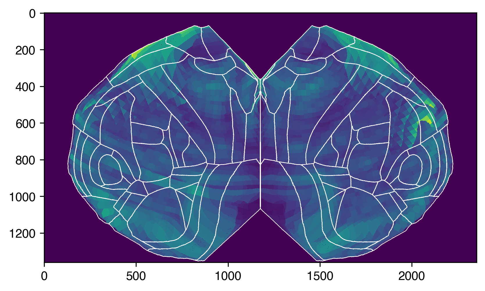
pdyn_projection_max = proj_bf.project_volume(pdyn_energy_upscale)
plt.imshow(
    pdyn_projection_max.T, # transpose so that the rostral/caudal direction is up/down
    interpolation='none',
    cmap='viridis',
)

for k, boundary_coords in bf_left_boundaries.items():
    plt.plot(*boundary_coords.T, c="white", lw=0.5)
for k, boundary_coords in bf_right_boundaries.items():
    plt.plot(*boundary_coords.T, c="white", lw=0.5)